Teaching a Neural Network to recognise Handwriting

Though machines have historically been unable to match human vision, recent advances in deep learning have made it possible to build neural networks that can recognize objects, faces, and text with incredible accuracy.

The focus of this post is to implement a small subsection of object recognition—digit recognition. We will create a simple application that recognizes handwritten digits and outputs the prediction. This app will run directly on the browser without any installations. We will use Google Colab for training and refining the model, and then deploy it on the browser using TensorFlowJS.

Code and Demo

You can find the code on Github and test the notebook on Google Colab using this link.

Project Pipeline

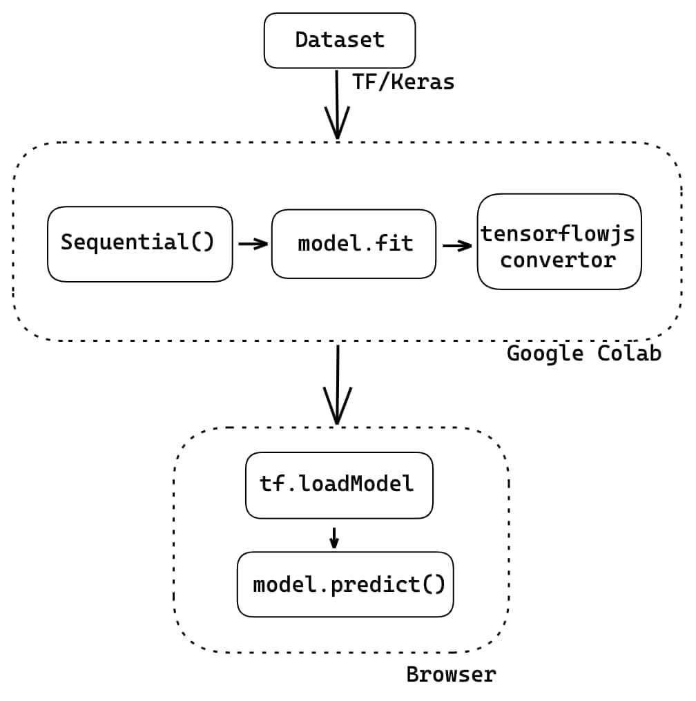
The pipeline for our project looks like this:

Import the dataset using TensorFlow Keras APIs
Training and testing different model architectures on GPU using Google Colab
Exporting the trained model for use in browser
Making predictions in the browser using TensorFlowJS

Loading and Visualising the dataset

We will be using MNIST which is one of the most common datasets used for image classification. It contains a set of 70k handwritten digits resized into a size of 28x82 pixels. The data is divided into a set of 60k training and 10k test images.

TensorFlow and Keras allow us to import and download the MNIST dataset directly from their API. Therefore, we start with the following lines to import MNIST dataset and check its shape.

python

(training_images, training_labels), (test_images, test_labels) = tf.keras.datasets.mnist.load_data()

print('Shape of training_images dataset', training_images.shape)
print('Shape of training_labels', training_labels.shape)
print('Shape of training_images dataset', test_images.shape)
print('Shape of test_labels', test_labels.shape)

# outputs
# Shape of training_images dataset (60000, 28, 28)
# Shape of training_labels (60000,)
# Shape of training_images dataset (10000, 28, 28)
# Shape of test_labels (10000,)

Here, 60000 & 10000 represents the number of images in the training and testing dataset respectively, and (28, 28) represents the size of the image.

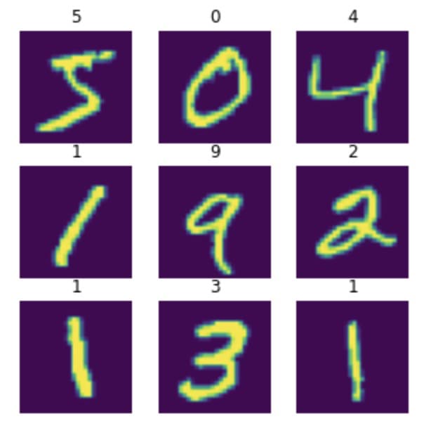
Converting these pixel values to image representation reveals the handwritten numbers which we will be training our model on.

Normalizing the Data

The images comprise matrices of pixel values. Color images have an array of pixel values for each color channel in RGB. Although these pixel values can be presented directly to neural network models in their raw format, this can result in slower training of the model. Hence, we will standardize values to be in the 0-1 by dividing the RGB codes to 255 (which is the maximum RGB code minus the minimum RGB code).

It's important that the training set and the testing set be preprocessed in the same way. Hence we will apply the same normalization on the testing dataset as well.

python


# Making sure that the values are float so that we can get decimal points after division
training_images = training_images.astype('float32')
test_images = test_images.astype('float32')


# Normalizing the RGB codes by dividing it to the max RGB value.
training_images = training_images / 255.0
test_images = test_images / 255.0

Training a Deep Neural Network

We will start with a very basic Neural Network which has 2 dense layers. The first layer consisting with flattening the 2-dimensional vector to a single dimension. Since we want to predict 0-9 digits (classes), we keep the last layer with 10 outputs activated by a softmax activation. This normalizes the values from the ten output nodes such that:

all the values are between 0 and 1, and
the sum of all ten values is 1

python

# define model
model = tf.keras.models.Sequential([
    tf.keras.layers.Flatten(input_shape=(28, 28)),
    tf.keras.layers.Dense(128, activation='relu'),
    tf.keras.layers.Dense(10, activation='softmax')
])

# compile
model.compile(optimizer='adam', loss='sparse_categorical_crossentropy', metrics=['accuracy'])

# train
history = model.fit(training_images, training_labels, epochs=20, validation_data=(test_images, test_labels))

Training this for 20 epochs results in a 97.98% accuracy on the validation set.

Although we achieved a pretty good accuracy, this is not the correct way to work on image processing/computer vision problems. The meaning of what a picture represents is through a combination of pixels that are adjacent to each other. But by flattening the 28x28 pixel image, we have obfuscated this information. Next, we will see Convolutional Neural Networks which are best suited for computer vision problems.

Training a Convolutional Neural Network

To overcome the loss of information we did in DNN, we will use CNN which is very well suited to preserve the spatial relationships between adjacent pixels. A typical CNN design begins with feature extraction and finishes with final image classification.

Feature extraction is performed by alternating convolution layers with subsampling layers
Classification is performed with dense layers followed by a final softmax layer

Also, to be able to use the dataset in Keras API, we need 4-dims NumPy arrays. Hence, we will also need to reshape the data before feeding to the models.

python

# Reshaping the array to 4-dims so that it can work with the Keras API
training_images = training_images.reshape(training_images.shape[0], 28, 28, 1)
test_images = test_images.reshape(test_images.shape[0], 28, 28, 1)

print('training_images shape:', training_images.shape)
print('test_images shape:', test_images.shape)

# output:
# training_images shape: (60000, 28, 28, 1)
# test_images shape: (10000, 28, 28, 1)

We will start with a standard CNN model with a Convolutional layer with 64-dimensional filter followed by a Pooling layer. Similar to the DNN, the last layer will be a Dense layer containing 10 outputs activated by a softmax activation to predict the 10 classes.

python

# define model
model = tf.keras.models.Sequential([
    tf.keras.layers.Conv2D(64, kernel_size=(3,3), activation='relu', input_shape=(28, 28, 1)),
    tf.keras.layers.MaxPooling2D(pool_size=(2, 2)),
    tf.keras.layers.Flatten(),
    tf.keras.layers.Dense(128, activation='relu'),
    tf.keras.layers.Dense(10, activation='softmax')
])
model.summary()

# compile
model.compile(optimizer='adam', loss='sparse_categorical_crossentropy', metrics=['accuracy'])

# train
history = model.fit(training_images, training_labels, epochs=20, validation_data=(test_images, test_labels))

Training this model for 20 epochs results in a 98.33% accuracy on the validation set.

As evident from the graphs, the accuracy of this model remains the same after 12-13 epochs. Even the validation loss is not a smooth progression. One of the primary reasons for this is that our model is overfitting on the data. To fix this we can try our some better feature extraction by introducing some more convolutional subsampling pairs and adding some dropout layers. The steps on how we arrived to this layer configuration is explained in detail in this notebook.

python

# define model
model = tf.keras.models.Sequential([
    layers.Conv2D(24,kernel_size=5,padding='same',activation='relu',input_shape=(28,28,1)),
    layers.MaxPooling2D(),
    tf.keras.layers.Dropout(0.2),
    layers.Conv2D(48,kernel_size=5,padding='same',activation='relu'),
    layers.MaxPooling2D(),
    layers.Conv2D(64,kernel_size=5,padding='same',activation='relu'),
    layers.MaxPooling2D(),
    tf.keras.layers.Dropout(0.4),
    tf.keras.layers.Flatten(),
    tf.keras.layers.Dense(128, activation='relu'),
    tf.keras.layers.Dense(10, activation='softmax')
])

# compile model
model.compile(optimizer='adam', loss='sparse_categorical_crossentropy', metrics=['accuracy'])

# train model
history = model.fit(training_images, training_labels, epochs=10, validation_data=(test_images, test_labels), verbose=0)

Training this improvised model for 20 epochs results in a 99.38% accuracy on the validation set. Also, as evident from the converging graphs, we have reduced the overfitting considerably.

Training Summary

This is the final summary of the few model architectures we have covered so far.

Architecture	Training time on GPU (20 epochs)	Training Accuracy	Validation Accuracy
DNN - 1	80s	99.8	97.98
CNN - 1	200s	99.93	98.34
CNN - 2	220s	99.54	99.39

In just ~200 seconds of training, we have achieved state-of-the-art results by making our model recognise unseen data and interpreting the handwritten digits with an accuracy of over 99%.

There are few more ways which we can try to improve the model accuracy. We can play with tuning the hyper-parameters, try out image augmentation to increase the data set, and make use of a pre-trained model to apply conceptes of transfer learning. Covering all of these will be not in the best interest of this post. For now, we can take this final model combination and expose it to some real-time data!

Preparing model for Web format

Till now, we have a model that is able to recognize digits with pretty good accuracy. But this model is still inside google colaboratory. To test this model with some real-world examples, we need to deploy it. One deployment strategy is to export the model to a web understandable format and provide it data via a web application.

TensorFlow provides a model convertor to convert Keras and TensorFlow models so that it can be used in a Javascript runtime. We convert the model and host the final model artefacts so that it can be downloaded in a web browser.

python

# install tensorflowjs python package
!pip install tensorflowjs

# save the current model as a keras HDF5 file format
model.save('keras.h5')

# convert the model
!mkdir model_js
!tensorflowjs_converter \
    --input_format=keras
    keras.h5  #/path/to/saved_model
    model_js/ #/path/to/output_dir

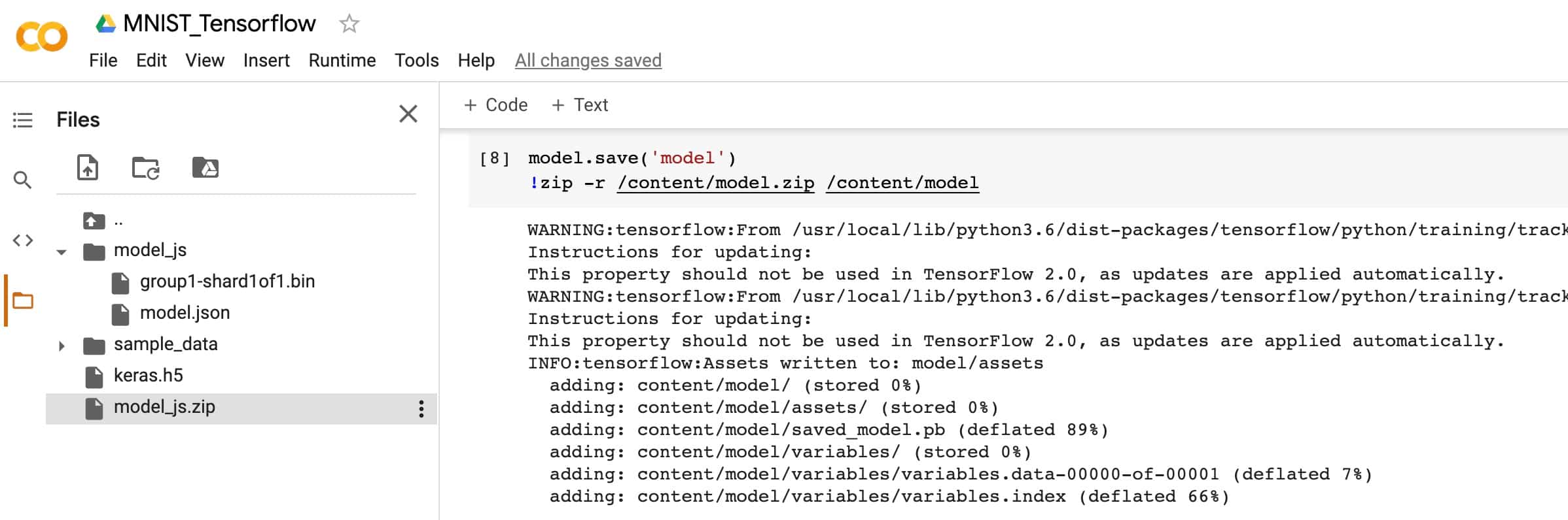
# zip all the relevant files so that we get a single downloadable file
!zip -r model_js.zip model_js

# download the zip file
from google.colab import files
files.download('model_js.zip')

The conversion script produces 2 types of file

model.json - dataflow graph and weight manifest file
group1-shard\*of\* - A group of binary weight files called shards. Each shard file is small in size for easier browser caching. The number of shards depends on the initial model.

Files generated during model export

To further validate if the conversion was correct, we can use the Neutron Visualiser to confirm the model architecture.

Model Summary

Web Client Application

So far, we have successfully trained a model on GPU and optimised the architecture so that we get good accuracy on unseen data. Then, we converted this model so that it can be run inside a browser javascript runtime. We can now load it into the browser via TensorFlowJS and make predictions.

javascript

const tf = require('@tensorflow/tfjs');

// this will load the model and the weights
const model = await tf.loadLayersModel('MODEL_URL');
const prediction = model.predict(tensor);

Pixels to Tensor

To create a similar Handwriting prediction environment, we can setup an HTML Canvas and enable freehand writing on it. Then we can convert this embedded pixel information inside our Canvas to tensor which our model understands. To recap, here’s what our trained model understands and works upon:

images of size 28x28 pixels
containing a single channel
normalised to values between 0-1

Similarly, our Canvas-to-Tensor conversion steps will be as follows:

Our canvas is 300x300 pixels. So we need to resize and convert the drawing back to 28x28 pixels.
- Convert the initial drawing to an Image using the Canvas.toDataURL() method.
- Redraw this image back on the canvas but resize it to 28x28. We can do this by calling the CanvasRenderingContext2D.drawImage() method and specifying the new dimensions in the arguments
Extract the pixel information from this smaller image by the CanvasRenderingContext2D.getImageData() function.
- The getImageData method returns an ImageData interface. This contains the image pixel data in form of an array. The data is in the RGBA order, with integer values between 0 and 255. i.e each pixel is represented as [0-255, 0-255, 0-255, 0-255]
- Since we need data from a single channel, we will extract the values contained in the Blue channel.
Finally, we normalise the values by dividing it by 255.

javascript

// EXTRACT: convert the drawn canvas to a image's Data URL representation
const img = new Image();
img.src = canvas.toDataURL('image/png');

img.onload = function () {
  // RESIZE: re-draw this image again on the same canvas in a 28x28 size
  context.drawImage(img, 0, 0, 28, 28);

  // NORMALIZE: Extract information from one channel (blue in our case)
  // and divide it with 255 to normalize it
  const data = context.getImageData(0, 0, 28, 28).data;
  const input = [];
  for (var i = 0; i < data.length; i += 4) {
    input.push(data[i + 2] / 255);
  }

  // Send the final JS array for prediction
  predict(input);
};

Finally we can convert this Array into a Tensor and reshape it in the correct form.

javascript

function predict(input) {
  const input_tensor = tf.tensor(input).reshape([1, 28, 28, 1]);
  const prediction_probs = await model.predict([input_tensor]).array();
}

The prediction will be an array of probabilities for each number. We pick the number which the model has assigned the maximum probability.

javascript

const maxProbability = Math.max(...prediction_probs);
const finalPrediction = predictionProbs.indexOf(maxProbability);

Demo

Combining everything, here's a working demo of the handwriting recogniser we have put together. Please try it out!

Please draw something to load Model and start the prediction